Review of AI (HITSZ) 含22年真题回顾
Review of AI (HITSZ)含22年真题回顾
1. Introduction
-
What is AI
AI is categorized into four types
- Systems that think like humans
- Systems that think rationally
- Systems that act like humans
- System that act rationally
The textbook advocates “acting rationally”.
-
What is Turing test approach
A test based on indistinguishability from undeniably intelligent entities and human beings. The computer passes the test if a human interrogator, after posing some written questions, cannot tell whether the written responses come from a person or not.
2. Intelligent Agents
-
What is agent
Anything that can be viewed as perceiving its environment through sensors and acting upon that environment through its actuators to maximize progress towards its goals.
PAGE: perceiving, environment, sensors, goals
-
What is rational agent
A rational agent chooses whichever action maximizes the expected value of the performance measure given the percept sequence to date and prior environment knowledge.
-
What is four elements of rational agents
PEAS
- Performance measure
- Prior environment knowledge
- Actions
- Sensors
-
Examples of rational agent and its elements
Medical diagnosis system
- Performance measure: Healthy patient, minimize costs, lawsuits.
- Environment: Patient, hospital, staffs
- Actuators: Screen display (questions, tests, diagnoses, treatments)
- Sensors: Keyboard (entry of symptoms, patient’s answer)
Part-picking robot
- Performance measure: Percentage of parts in correct bins (工具抽屉)
- Environment: Conveyor belt with parts, bins
- Actuators: Jointed arm and hand
- Sensors: Camera, joint angle sensors
Interactive English tutor
- Performance measure: Maximize student’s score on test
- Environment: Set of students
- Actuators: Screen display (exercises, suggestions, corrections)
- Sensors: Keyboard
-
Agent structure
agent = architecture + program
-
Agent program components
Atomic, Factored and Structured.
Explanation:
-
Atomic: An atomic representation is one in which each state is treated as a black box.
Example:
atomicState == goal: Y/N
Explanation:
Y/N is the only question we can ask to a black box
-
Factored: A factored representation is one in which the states are defined by set of features.
Example:
factoredState{18} == goal{42}: N // Is goal reached?
diff( goal{42}, factoredState{18}) = 24 // How much is difference?
// some other questions.Explanation:
The simplest factored state must have at least one feature (of some type), that gives us ability to ask more questions. Normally it defines quantitative difference between states. The example has one feature of integer type.
-
Structured: A structured representation is one in which the states are expressed in form of objects and relations between them. Such knowledge about relations called facts.
Example:
11grade@schoolA{John(Math=A-), Marry(Music=A+), Job1(doMath)…} == goal{50% ready for jobs}
Explanation:
The key here - structured representation, allows higher level of formal logical reasoning at the search.
-
-
Agent types
- Rationality: A property of agents that choose actions that maximize their expected utility, given the percepts to date.
- Autonomy: A property of agents whose behavior is determined by their own experience rather than solely by their initial programming.
- Reflex agent: an agent whose action depends only on the current percept.
- Model-based agent: an agent whose action is derived directly from an internal model of the current world state that is updated over time.
- Goal-based agent: an agent that selects actions that it believes will achieve explicitly represented goals.
- Utility-based agent: an agent that selects actions that it believes will maximize the expected utility of the outcome state.
- Learning agent: an agent whose behavior improves over time based on its experience.
3. Problem Define and Uniformed Searching
3.1 Problem Define
-
How to define a problem (5 items)
- State description: define the state of the given problem
- Initial State: the agent starts in.
- Actions/Successor functions: a description of the possible actions available to the agent.
- Goal test: determines if a given state is a goal state.
- Path cost: assigns a numeric cost to each paths (solutions).
-
Evaluation of search strategies
Note that:
-
b
b
b: maximum branching factor of the search tree -
d
d
d: depth of the least-cost solution -
m
m
m: maximum depth of the state space
- Completeness: does it always find a solution if one exists?
- Time complexity: how many number of nodes are generated?
- Space complexity: the maximum number of nodes in memory?
- Optimally: does it always find a least-cost solution?
-
3.2 Uniformed Searching (无信息搜索)
3.2.1 Search Algorithms
The basic framework of uniformed searching is (if it is a graph, then maintain a closed set):
def search(problem, fringe): -> a solution or falure
	fringe.insert(make-node(problem.initial-state))
    while:
        if fringe is empty:
            return fauilre
        node = fringe.pop()
        if problem.goal-test(node.state):
            return node
        fringe.insertall(expand(node,problem))

def expand(node, problem):
	succesors = []
    for action, state in Successor-fn(problem, node.state):
        s = make-node(state)
        s.parent = node
        s.action = action
        s.path-cost = node.path-cost + step-cost(node, action, s)
        s.depth = node.depth + 1
        succesors.append(s)
    return successors
-
Breadth-first search
Fringe is a FIFO queue. Nodes are appended at the end of the fringe.
-
Uniform-cost search
Fringe is a Priority queue.
-
Depth-first search
Fringe is a FILO stack. Nodes are inserted at the head of the fringe.
-
Depth-limited search
DFS with depth limit
l
l
l. That is to say, nodes at depth
l
l
l have no successors.
-
Iterative deepening search
Run depth-limited search iteratively unless find a solution. Otherwise, dead loop.
3.2.2 Measurements
| BFS | UCS | DFS | DLS | IDS | |
|---|---|---|---|---|---|
| Completion |
Y e s a Yes^a Yesa |
Y e s a , b Yes^{a,b} Yesa,b |
No | No | Yes |
| Time |
O ( b d + 1 ) O(b^{d+1}) O(bd+1) |
O ( b ⌈ 1 + C ∗ / ϵ ⌉ ) O(b^{\lceil 1+C^*/\epsilon \rceil}) O(b⌈1+C∗/ϵ⌉) |
O ( b m ) O(b^m) O(bm) |
O ( b l ) O(b^l) O(bl) |
O ( b d ) O(b^d) O(bd) |
| Space |
O ( b d + 1 ) O(b^{d+1}) O(bd+1) |
O ( b ⌈ 1 + C ∗ / ϵ ⌉ ) O(b^{\lceil 1+C^*/\epsilon \rceil}) O(b⌈1+C∗/ϵ⌉) |
O ( b m ) O(bm) O(bm) |
O ( b l ) O(bl) O(bl) |
O ( b d ) O(bd) O(bd) |
| Optimal |
Y e s c Yes^c Yesc |
Yes | No | No |
Y e s c Yes^c Yesc |
NOTE:
-
Y
e
s
a
Yes^a
Yesa: Completion if branch is finite.
-
Y
e
s
b
Yes^b
Yesb: Completion if step costs are non-negative (i.e., no-circle).
-
Y
e
s
c
Yes^c
Yesc: Optimal if step costs are the identical.
-
b
b
b: maximum branching factor of the search tree
-
d
d
d: depth of the least-cost solution
-
m
m
m: maximum depth of the state space
-
l
l
l: depth limit
4. Informed Search
4.1 Basic concepts
-
Heuristic function: denoted as
h
(
n
)
h(n)
h(n), which means the estimated cost of the cheapest path from node
n
n
n to a goal node.
-
Greedy best-first: Greedy best-first search tries to expand the node that is closest to the goal, on the grounds that this is likely to lead to a solution quickly. Thus, it evaluates nodes by using just the heuristic function:
f
(
n
)
=
h
(
n
)
f(n)=h(n)
f(n)=h(n)
- Complete: No. But can be complete in finite state space with repeated-state checking.
- Time:
O
(
b
m
)
O(b^m)
O(bm) - Space:
O
(
b
m
)
O(b^m)
O(bm) - Optimal: No
-
Evaluation function:
f
(
n
)
=
g
(
n
)
+
h
(
n
)
f(n) = g(n) +h(n)
f(n)=g(n)+h(n). Where
g
(
n
)
g(n)
g(n) is the so-far cost to reach
n
n
n,
h
(
n
)
h(n)
h(n) is the estimated cost from
n
n
n to the goal.
-
Admissible: A heuristic
h
(
n
)
h(n)
h(n) is admissible if for every node
n
n
n,
h
(
n
)
≤
h
∗
(
n
)
h(n)\le h^*(n)
h(n)≤h∗(n), where
h
∗
(
n
)
h^*(n)
h∗(n) is the true cost to reach the goal state from
n
n
n.
-
Consistency: A heuristic is consistent if for every node
n
n
n, every successor
n
′
n'
n′, generated by any action
a
a
a, we have
h
(
n
)
≤
c
(
n
,
a
,
n
′
)
+
h
(
n
′
)
h(n)\le c(n,a,n') + h(n')
h(n)≤c(n,a,n′)+h(n′)
Thus,
f
(
n
′
)
=
g
(
n
′
)
+
h
(
n
′
)
=
g
(
n
)
+
c
(
n
,
a
,
n
′
)
+
h
(
n
′
)
≥
g
(
n
)
+
h
(
n
)
≥
f
(
n
)
f(n')=g(n')+h(n')=g(n)+c(n,a,n')+h(n')\ge g(n)+h(n)\ge f(n)
f(n′)=g(n′)+h(n′)=g(n)+c(n,a,n′)+h(n′)≥g(n)+h(n)≥f(n)
-
If a heuristic function is consistency then it is admissible
Proof by induction.
-
Dominance (占优问题): If
h
2
(
n
)
≥
h
1
(
n
)
h_2(n)\ge h_1(n)
h2(n)≥h1(n) for all
n
n
n (Assume
h
2
(
x
)
h_2(x)
h2(x) and
h
1
(
x
)
h_1(x)
h1(x) are both admissible). Then
h
2
h_2
h2 dominates
h
1
h_1
h1, and
h
2
h_2
h2 is better for search.
4.2 A* search
- A* used in tree search is optimal if
h
(
n
)
h(n)
h(n) is admissible. - A* used in graph search is optimal if
h
(
n
)
h(n)
h(n) is consistent. - Complete: Yes (unless there are infinitely many nodes with
f
≤
f
(
G
)
f\le f(G)
f≤f(G)) - Time: Exponential
- Space: Keeps all nodes in memory
- A* expands all nodes with
f
(
n
)
<
C
∗
f(n)<C^*
f(n)<C∗ - A* expands some nodes with
f
(
n
)
=
C
∗
f(n)=C^*
f(n)=C∗ - A* expands no nodes with
f
(
n
)
>
C
∗
f(n) > C^*
f(n)>C∗
- A* expands all nodes with
4.3 Local Search Algorithms
-
Hill-climbing Search
- Steepest-ascent (最陡峭上升法)
- Random-restart
- First-choice
-
Simulated annealing
def simulated_annealing(problem, schedule) current = make-node(problem.initial-state) for t in range(1, MAX): Temperature = schedule[t] if T = 0: return current successor = randomly choose successor of current E = successor.value - current.value if E > 0: current = successor else: with probablity e ** (E/T), current = successor -
Local beam search
Keep
k
k
k states instead of 1; choose top
k
k
k of all their successors. These successors are not the same, as
k
k
k searches run in parallel. In a random-restart search, each search process runs independently of the others. In a local beam search, useful information is passed among the k parallel search threads.
-
Genetic algorithms
- Start with
k
k
k randomly generated states. - Produce the next generation of states by selection, crossover, and mutation.
- Start with
5. Constrained Satisfaction Problem
5.1 Basic Concepts
- Definition of CSP
- State is defined by variables
X
i
X_i
Xi with values from domainD
i
D_i
Di. - Goal tests is a set of constraints specifying allowable combinations of values for subsets of variables.
- A constraint satisfaction problem (or CSP) is defined by a set of variables,
X
1
,
X
2
,
.
.
.
,
X
n
X_1, X_2,. . .,X_n
X1,X2,...,Xn, and a set of constraints,C
1
,
…
,
C
m
C_1,…, C_m
C1,…,Cm,. Each variableX
i
Xi
Xi has a domainD
i
Di
Di of possible values. Each constraintC
i
Ci
Ci involves some subset of the variables and specifies the allowable combinations of values for that subset.
- State is defined by variables
5.2 Four search methods of CSP
- Backtracking: DFS with backtracks.
- MRV: Choosing the variable with the fewest “legal” values is called the minimum remaining values (MRV) heuristic.
- Forward Checking/Least Constrain
- Forward Check: Whenever a variable
X
X
X is assigned, the forward checking process looks at each unassigned variableY
Y
Y that is connected toX
X
X by a constraint and deletes fromY
Y
Y’s domain any value that is inconsistent with the value chosen forX
X
X. - Least Constraining Value: The one that rules out the fewest values in the remaining variables.
- Forward Check: Whenever a variable
- Arc Consistency Algorithm (AC-3): AC-3 puts back on the queue every arc
(
X
k
,
X
i
)
(X_k, X_i)
(Xk,Xi) whenever any value is deleted from the domain ofX
i
X_i
Xi, even if each value ofX
k
X_k
Xk is consistent with several remaining values ofX
i
X_i
Xi.-
X
→
Y
X\rightarrow Y
X→Y is consistent iff for every valuex
x
x ofX
X
X, there is some allowedy
y
y. - If
X
X
X loses a value, neighbors ofX
X
X, say,Y
i
Y_i
Yi,Y
i
→
X
Y_i\rightarrow X
Yi→X, should be rechecked.
-
6. Game
6.1 Game Types
| Single-player | Multi-player |
|---|---|
| Zero-sum | Non-zero-sum |
| Deterministic | Non-deterministic |
| Perfect information | Imperfect information |
| Deterministic | Chance | |
|---|---|---|
| Perfect information | Chess, checkers(西洋跳棋), go, Othello | Backgammon西洋双陆棋, monopoly |
| Imperfect information | Stratego, JunQi | Bridge, poker, scrabble拼字游戏, nuclear war |
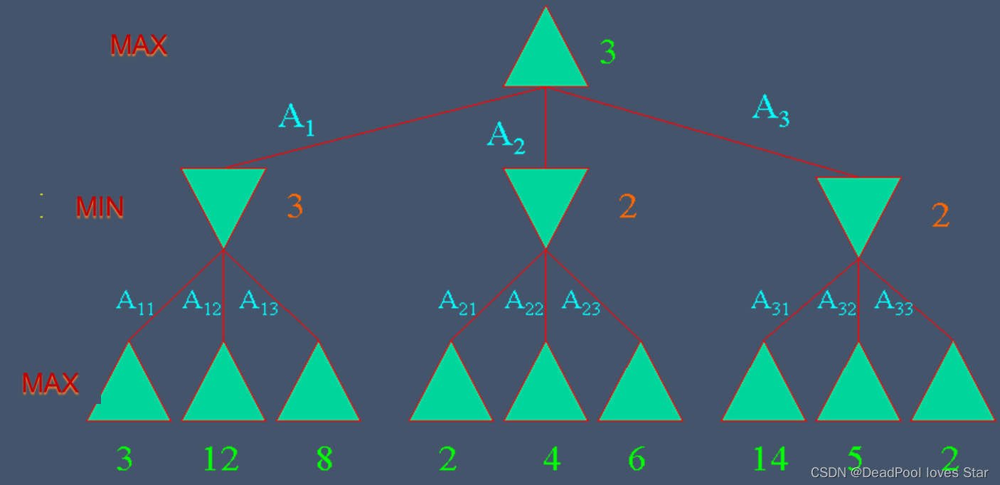
6.2 Mini-max Decision Algorithm
6.2.1 Strategy
- Optimal strategy for MAX.
- Generate the whole game tree.
- Calculate the value of each terminal state based on the utility function.
- Calculate the utilities of the higher-level nodes starting from the leaf nodes up to the root.
- MAX selects the value with the highest node.
- MAX assumes that MIN in its move will select the node that minimizes the value.
6.2.2 Mini-max algorithm
def minimax-decision(state):
    v = max-value(state)
    return the action in successors(state) with value v

def max-value(state):
    if terminal-test(state):
        return utility(state)
    v = MIN
    # select the maximam value
    for action, successor in successors(state):
        v = max(v, min-value(successor))
    return v

def min-value(state):
    if terminal-test(state):
        return utility(state)
    v = MAX
    for action, successor in successors(state):
        v = min(v, max-value(successor))
    return v
6.3 Alpha-Beta Pruning
Check Alpha-Beta剪枝算法(人工智能)_哔哩哔哩_bilibili
def alpha-beta-search(state):
    v = max-value(state, MIN, MAX)
    return the action in successors(state) with value v

def max-value(state, alpha, beta):
    if terminal-test(state):
        return utility(state)
    v = MIN
    # select the maximam value
    for action, successor in successors(state):
        v = max(v, min-value(successor, alpha, beta))
        if v >= beta:
            return v
        alpha = max(alpha, v)
    return v

def min-value(state, alpha, beta):
    if terminal-test(state):
        return utility(state)
    v = MAX
    for action, successor in successors(state):
        v = min(v, max-value(successor, alpha, beta))
        if v <= alpha:
            return v
        beta = min(beta, v)
    return v
7. Logic Agents
7.1 Basic Concepts
-
Entailment/Inference
- Entailment means that one thing follows from another:
K
B
⊨
α
KB \vDash α
KB⊨α - Knowledge base
K
B
KB
KB entails sentenceα
α
α if and only ifα
α
α is true in all worlds whereK
B
KB
KB is true- E.g., the KB containing “the Giants won” and “the Reds won” entails “Either the Giants won or the Reds won”
- E.g., x+y = 4 entails 4 = x+y
- Entailment is a relationship between sentences (i.e., syntax) that is based on semantics
-
M
(
K
B
)
⊆
M
(
α
)
M(KB)\subseteq M(\alpha)
M(KB)⊆M(α), whereM
(
K
B
)
M(KB)
M(KB) denotes the set of models that makeK
B
KB
KB true.
- Entailment means that one thing follows from another:
-
Completeness/Soundness
-
K
B
⊢
i
α
KB\vdash_i\alpha
KB⊢iα means: sentenceα
\alpha
α can be derived fromK
B
KB
KB by procedurei
i
i. - Soundness:
i
i
i is sound if wheneverK
B
⊢
i
α
KB\vdash_i\alpha
KB⊢iα, it is also true thatK
B
⊨
α
KB\vDash\alpha
KB⊨α - Completeness:
i
i
i is complete if wheneverK
B
⊨
α
KB\vDash\alpha
KB⊨α, it is also true thatK
B
⊢
i
α
KB\vdash_i\alpha
KB⊢iα
-
-
Syntax/Semantics
Syntax defines the sentences in the language
- Propositional logic (命题逻辑) is the simplest logic – illustrates basic ideas
- The proposition symbols P1, P2, etc. are sentences
- If
S
S
S is a sentence,¬
S
\neg S
¬S is a sentence (negation) - If
S
1
S_1
S1 andS
2
S_2
S2 are sentences,S
1
∧
S
2
S_1 \land S_2
S1∧S2 is a sentence (conjunction) - If
S
1
S_1
S1 andS
2
S_2
S2 are sentences,S
1
∨
S
2
S_1 \lor S_2
S1∨S2 is a sentence (disjunction) - If
S
1
S_1
S1 andS
2
S_2
S2 are sentences,S
1
⇒
S
2
S_1 \Rightarrow S_2
S1⇒S2 is a sentence (implication) - If
S
1
S_1
S1 andS
2
S_2
S2 are sentences,S
1
⇔
S
2
S1 \Leftrightarrow S2
S1⇔S2 is a sentence (biconditional)
- If
Semantics define the “meaning” of sentences: define truth of a sentence in a world
-
Logically equivalent
Two sentences are logically equivalent iff true in same models. That is to say:
α
≡
β
α ≡ \beta
α≡β iff
α
⊨
β
α\vDash β
α⊨β and
β
⊨
α
β\vDash α
β⊨α.
NOTE:
-
α
⇒
β
≡
¬
α
∨
β
\alpha \Rightarrow \beta ≡ \neg\alpha\lor \beta
α⇒β≡¬α∨β
-
-
Validity/Satisfiability
-
A sentence is valid if it is true in all models,
e.g., True,
A
∨
¬
A
A\lor \neg A
A∨¬A,
A
⇒
A
A \Rightarrow A
A⇒A,
(
A
∧
(
A
⇒
B
)
)
⇒
B
(A \land (A \Rightarrow B)) \Rightarrow B
(A∧(A⇒B))⇒B
Validity is connected to inference via the Deduction Theorem:
K
B
⊨
α
KB \vDash \alpha
KB⊨α iff (
K
B
⇒
α
KB \Rightarrow α
KB⇒α) is valid
-
A sentence is satisfiable if it is true in some model
e.g.,
A
∨
B
A\lor B
A∨B,
C
C
C
-
A sentence is un-satisfiable if it is true in no models
e.g.,
A
∧
¬
A
A\land \neg A
A∧¬A
Satisfiability is connected to inference via the following:
K
B
⊨
α
KB \vDash \alpha
KB⊨α iff (
K
B
∧
¬
α
KB \land \neg α
KB∧¬α) is un-satisfiable (i.e., (
¬
(
K
B
∧
¬
α
)
\neg (KB \land \neg α)
¬(KB∧¬α)) is valid, i.e., (
¬
K
B
∨
α
\neg KB\lor \alpha
¬KB∨α) is valid, )
-
7.2 Proof Methods
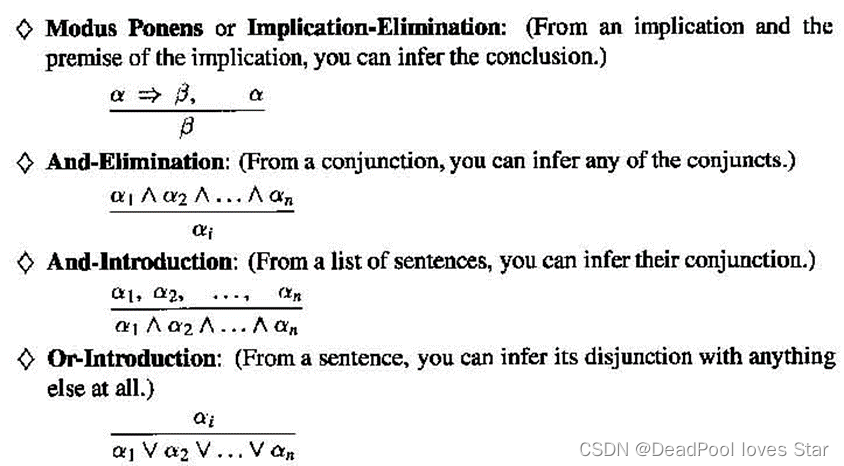
-
Inference rules
NOTE:
Modus ponens (肯定前件)
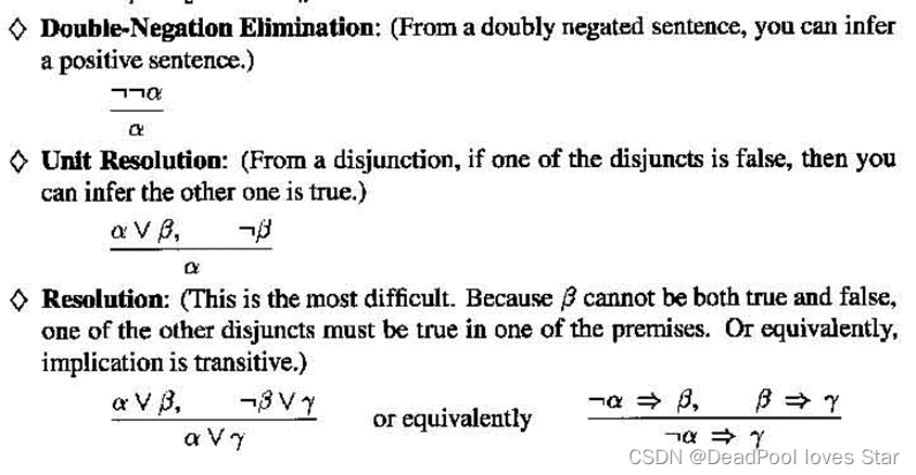
-
Resolution
-
Conjunctive Normal Form (CNF) (合取范式)
(
A
∨
B
)
∧
(
¬
B
∨
C
∨
D
∨
¬
E
)
(A\lor B) \land (\neg B\lor C \lor D\lor \neg E)
(A∨B)∧(¬B∨C∨D∨¬E)
-
Resolution
Before:
(
A
∨
B
)
∧
(
¬
B
∨
C
∨
D
∨
¬
E
)
(A\lor B) \land (\neg B\lor C \lor D\lor \neg E)
(A∨B)∧(¬B∨C∨D∨¬E)
After:
A
∨
C
∨
D
∨
¬
E
A \lor C \lor D\lor \neg E
A∨C∨D∨¬E
-
Conversion to CNF
-
Resolution Algorithm
Show
K
B
∧
α
KB\land \alpha
KB∧α is un-satisfiable.
-
Horn Form: Conjunction of Horn clauses (clauses with ≤ 1 positive literal)
-
Forward Chaining
-
Backward Chaining
-
Forward Chaining vs. Backward Chaining
- FC is data-driven, automatic, unconscious process
- BC is goal-driven, appropriate for problem-solving
-
8. Inference in First-Order Logic
8.1 Substitution and Unify
-
U
n
i
f
y
(
K
n
o
w
s
(
J
o
h
n
,
x
)
,
K
n
o
w
s
(
J
o
h
n
,
J
a
n
e
)
)
=
{
x
/
J
a
n
e
}
Unify(Knows(John,x),Knows(John,Jane))=\{x/Jane\}
Unify(Knows(John,x),Knows(John,Jane))={x/Jane} -
U
n
i
f
y
(
K
n
o
w
s
(
J
o
h
n
,
x
)
,
K
n
o
w
s
(
y
,
B
i
l
l
)
)
=
{
x
/
B
i
l
l
,
y
/
J
o
h
n
}
Unify(Knows(John,x),Knows(y,Bill))=\{x/Bill,y/John\}
Unify(Knows(John,x),Knows(y,Bill))={x/Bill,y/John} -
U
n
i
f
y
(
K
n
o
w
s
(
J
o
h
n
,
x
)
,
K
n
o
w
s
(
y
,
M
o
t
h
e
r
(
y
)
)
)
=
{
y
/
J
o
h
n
,
x
/
M
o
t
h
e
r
(
J
o
h
n
)
}
Unify(Knows(John,x),Knows(y,Mother(y)))=\{y/John,x/Mother(John)\}
Unify(Knows(John,x),Knows(y,Mother(y)))={y/John,x/Mother(John)} -
U
n
i
f
y
(
K
n
o
w
s
(
J
o
h
n
,
x
)
,
K
n
o
w
s
(
x
,
E
l
i
z
a
b
e
t
h
)
)
=
{
f
a
i
l
}
Unify(Knows(John,x),Knows(x,Elizabeth))=\{fail\}
Unify(Knows(John,x),Knows(x,Elizabeth))={fail}
8.2 Generalized Modus Ponens (GMP)
- Definite Clause: Disjunctions of literals of which exactly one is positive (肯定)
- A definite clause either is atomic or is an implication whose antecedent (前项) is a conjunction of positive literals and whose consequent (后项) is a single positive literal.
- Unlike propositional literals, FOL literals can include variables (universally quantified)
- Forward Chaining
- Backward Chaining
8.3 Resolution
- 消除蕴含
- 将
¬
\neg
¬内移 - 变量标准化(存在量词换名)
- 去除存在量词(变量Skolem化)
- 去除全称量词
- 将
∧
\land
∧分配到∨
\lor
∨中
9. Uncertainty
- Prior (Unconditional) probability is the degree of belief in the absence of any other information.
- Posterior (Conditional) probability is the degree of belief, given some evidence.
- Joint probability distribution for a set of random variables gives the probability of every atomic event on those random variables
- Likelihood probability is the likelihood of the data under each hypothesis.
- Enumeration
- Independence
- Bayes Rule
10. Bayesian networks
-
Definition
A simple, graphical notation for conditional independence assertions and hence for compact specification of full joint distributions
-
Semantics
-
Numeric semantic: full joint distribution of Bayesian networks
P
(
x
1
,
.
.
.
,
x
n
)
=
Π
i
=
1
n
P
(
x
i
∣
P
a
r
e
n
t
s
(
x
i
)
)
P(x_1,...,x_n)=\Pi_{i=1}^nP(x_i|Parents(x_i))
P(x1,...,xn)=Πi=1nP(xi∣Parents(xi))
-
Topological semantic: each node is independent of all others given its Markov blanket
Markov Blanket: Parents + Children + Children’s parents
-
-
Constructing Bayesian Networks
See if the new variable is independent of given variables.
-
Noisy-OR
Add a leak node as other unknown causes.
-
Inference tasks
-
Simple queries
P
(
X
i
∣
E
=
e
)
P(X_i|E=e)
P(Xi∣E=e)
-
Conjunctive queries
P
(
X
i
,
X
j
∣
E
=
e
)
=
P
(
X
i
∣
E
=
e
)
P
(
X
j
∣
X
i
,
E
=
e
)
P(X_i,X_j|E=e)=P(X_i|E=e)P(X_j|X_i,E=e)
P(Xi,Xj∣E=e)=P(Xi∣E=e)P(Xj∣Xi,E=e)
-
-
Exact Inference
-
Enumeration
P
(
B
∣
j
,
m
)
=
α
∑
e
∑
a
P
(
B
,
e
,
a
,
j
,
m
)
=
α
∑
e
∑
a
P
(
B
)
∗
P
(
e
)
∗
P
(
a
∣
B
,
e
)
∗
P
(
j
∣
a
)
∗
P
(
m
∣
a
)
=
α
P
(
B
)
∗
∑
e
P
(
e
)
∑
a
∗
P
(
a
∣
B
,
e
)
∗
P
(
j
∣
a
)
∗
P
(
m
∣
a
)
\begin{aligned} P(B|j,m) &=\alpha\sum_e\sum_aP(B,e,a,j,m)\\ &=\alpha\sum_e\sum_aP(B)*P(e)*P(a|B,e)*P(j|a)*P(m|a)\\ &=\alpha P(B)*\sum_eP(e)\sum_a*P(a|B,e)*P(j|a)*P(m|a) \end{aligned}
P(B∣j,m)=αe∑a∑P(B,e,a,j,m)=αe∑a∑P(B)∗P(e)∗P(a∣B,e)∗P(j∣a)∗P(m∣a)=αP(B)∗e∑P(e)a∑∗P(a∣B,e)∗P(j∣a)∗P(m∣a)
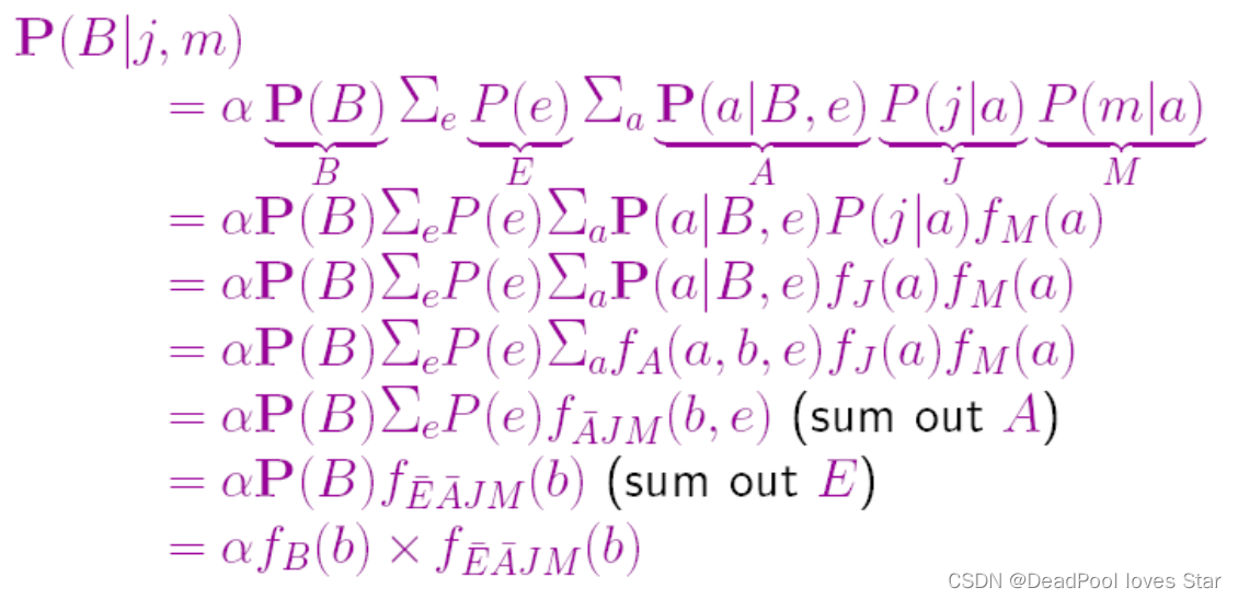
-
Variable elimination

-
-
Approximate Inference
-
Stochastic simulation
-
Sampling from an empty network
-
Rejection sampling: Selecting the samples agreeing with given evidence.
-
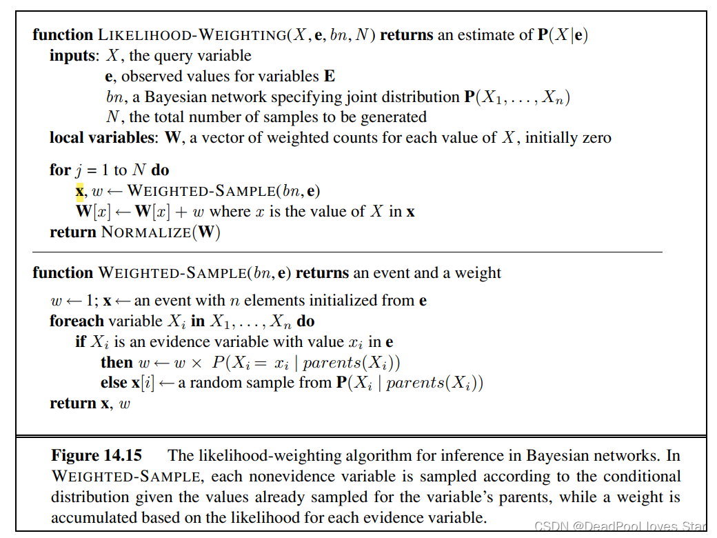
Likelihood weighting: Fix evidence variables, sample only nonevidence variables, and weight each sample by the likelihood it accords the evidence. Sample from parents.
-
-
Markov chain Monte Carlo
Sampling from Markov Blanket.
-

11. 2022年真题回顾
11.1 概念题
- Agent
- Rational Agent
- Goal-based Agent
- Utility-based Agent
- Model-based Agent
- Reflex Agent
11.2 大题
-
给三句话,用FOL表述。最后一个是每个爱动物的人都有一个人爱他
-
Game问题,很tricky,P1、P2用的不同效度函数,我的理解是P2让P1的效度少,P1让P2的效度少
-
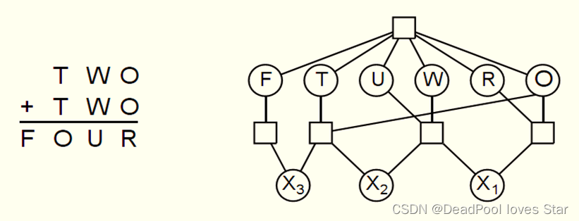
密码问题
-
A*,求最短路径
-
贝叶斯网络(性质、概念、没有计算)
-
贝叶斯网络中的拒绝采样与似然采样,看起来很复杂,做起来相对容易。需要熟悉似然采样的流程