深度学习速成版01—神经网络
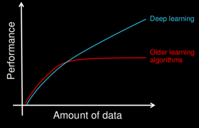
深度学习与机器学习的区别
- 机器学习的特征工程步骤是要靠手动完成的,而且需要大量领域专业知识
- 深度学习通常由多个层组成,它们通常将更简单的模型组合在一起,通过将数据从一层传递到另一层来构建更复杂的模型。通过大量数据的训练自动得到模型,不需要人工设计特征提取环节。
- 深度学习算法试图从数据中学习高级功能,这是深度学习的一个非常独特的部分。因此,减少了为每个问题开发新特征提取器的任务。适合用在难提取特征的图像、语音、自然语言领域
神经网络
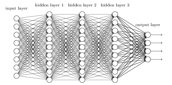
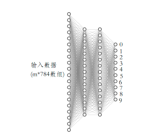
人工神经网络( Artificial Neural Network, 简写为ANN)也简称为神经网络(NN)。是一种模仿生物神经网络(动物的中枢神经系统,特别是大脑)结构和功能的 计算模型。经典的神经网络结构包含三个层次的神经网络。分别输入层,输出层以及隐藏层。
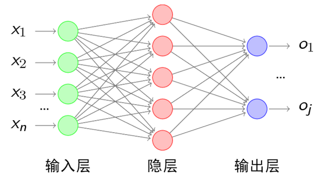
其中每层的圆圈代表一个神经元,隐藏层和输出层的神经元有输入的数据计算后输出,输入层的神经元只是输入。
神经网络的特点
- 每个连接都有个权值
- 同一层神经元之间没有连接
- 最后的输出结果对应的层也称之为
全连接层FC
那么为什么设计这样的结构呢?首先从一个最基础的结构说起,神经元。以前也称之为感知机。神经元就是要模拟人的神经元结构。
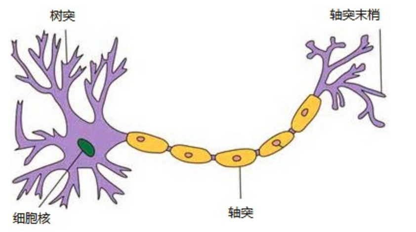
1943 年,McCulloch 和 Pitts 将上述情形抽象为上图所示的简单模型,这就是一直沿用至今的 M-P 神经元模型。把许多这样的神经元按一定的层次结构连接起来,就得到了神经网络。一个简单的神经元如下图所示,
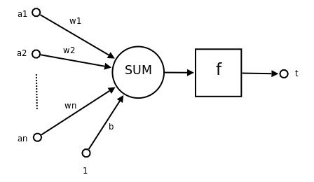
其中:
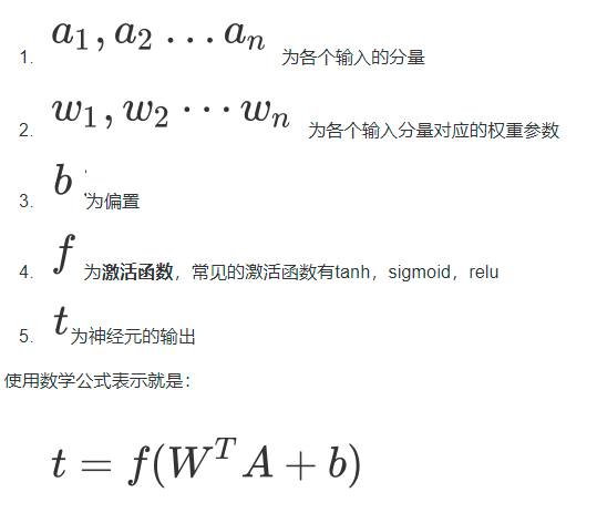
可见,一个神经元的功能是求得输入向量与权向量的内积后,经一个非线性传递函数得到一个标量结果。
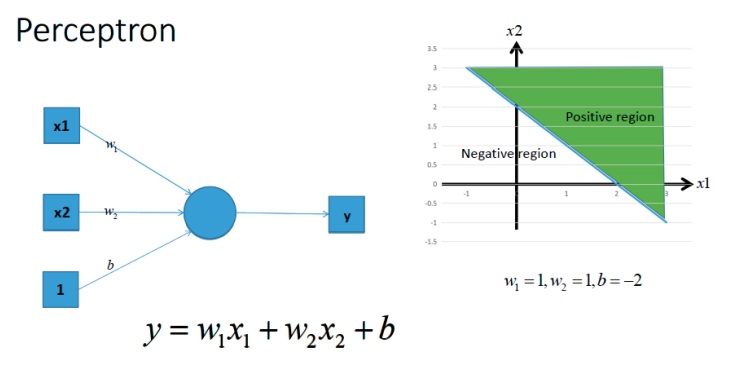
感知机(PLA: Perceptron Learning Algorithm))
感知机就是模拟这样的大脑神经网络处理数据的过程。感知机模型如下图:
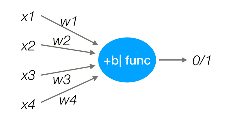
感知机是一种最基础的分类模型,类似于逻辑回归。感知机最基础是这样的函数,而逻辑回归用的sigmoid。这个感知机具有连接的权重和偏置
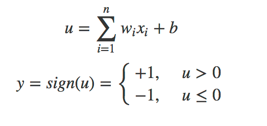
感知机的激活函数是符号函数:sign(z) = +1 (if z >=0) else -1
感知机的作用:
把一个n维向量空间用一个超平面分割成两部分,给定一个输入向量,超平面可以判断出这个向量位于超平面的哪一边,得到输入时正类或者是反类,对应到2维空间就是一条直线把一个平面分为两个部分。
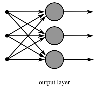
- 单层神经网络
是最基本的神经元网络形式,由有限个神经元构成,所有神经元的输入向量都是同一个向量。由于每一个神经元都会产生一个标量结果,所以单层神经元的输出是一个向量,向量的维数等于神经元的数目。示意图如下
多层神经网络
多层神经网络就是由单层神经网络进行叠加之后得到的,所以就形成了层的概念,常见的多层神经网络有如下结构:
- 输入层(Input layer),众多神经元(Neuron)接受大量输入消息。输入的消息称为输入向量。
- 输出层(Output layer),消息在神经元链接中传输、分析、权衡,形成输出结果。输出的消息称为输出向量。
- 隐藏层(Hidden layer),简称“隐层”,是输入层和输出层之间众多神经元和链接组成的各个层面。隐层可以有一层或多层。隐层的节点(神经元)数目不定,但数目越多神经网络的非线性越显著,从而神经网络的强健性(robustness)更显著。
示意图如下:
全连接层
全连接层:当前一层和前一层每个神经元相互链接,我们称当前这一层为全连接层。
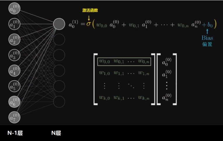
从上图可以看出,所谓的全连接层就是在前一层的输出的基础上进行一次
的变化(不考虑激活函数的情况下就是一次线性变化,所谓线性变化就是平移(+b)和缩放的组合(*w))
- 激活函数
在前面的神经元的介绍过程中我们提到了激活函数,那么他到底是干什么的呢?
假设我们有这样一组数据,三角形和四边形,需要把他们分为两类
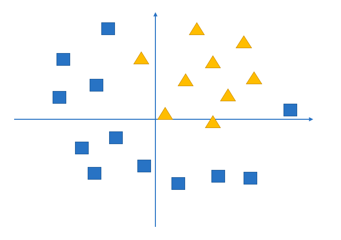
通过不带激活函数的感知机模型我们可以划出一条线, 把平面分割开
假设我们确定了参数w和b之后,那么带入需要预测的数据,如果y>0,我们认为这个点在直线的右边,也就是正类(三角形),否则是在左边(四边形)
但是可以看出,三角形和四边形是没有办法通过直线分开的,那么这个时候该怎么办?
可以考虑使用多层神经网络来进行尝试,比如在前面的感知机模型中再增加一层
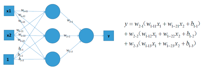
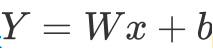
对上图中的等式进行合并,我们可以得到:

上式括号中的都为w参数,和公式
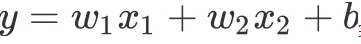
完全相同,依然只能够绘制出直线
所以可以发现,即使是多层神经网络,相比于前面的感知机,没有任何的改进。
但是如果此时,我们在前面感知机的基础上加上非线性的激活函数之后,输出的结果就不在是一条直线
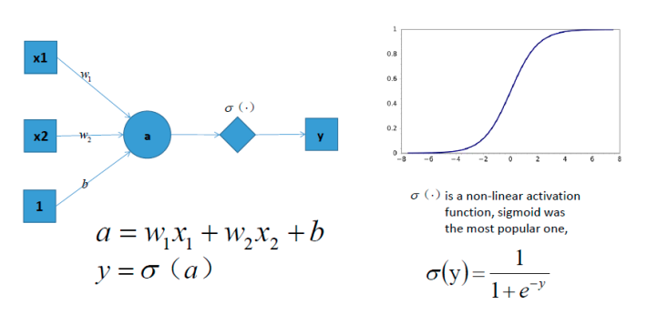
如上图,右边是sigmoid函数,对感知机的结果,通过sigmoid函数进行处理
如果给定合适的参数w和b,就可以得到合适的曲线,能够完成对最开始问题的非线性分割
所以激活函数很重要的一个作用就是增加模型的非线性分割能力
常见的激活函数有:
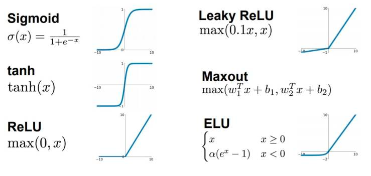
看图可知:
- sigmoid 只会输出正数,以及靠近0的输出变化率最大
- tanh和sigmoid不同的是,tanh输出可以是负数
- Relu是输入只能大于0,如果你输入含有负数,Relu就不适合,如果你的输入是图片格式,Relu就挺常用的,因为图片的像素值作为输入时取值为[0,255]。
激活函数的作用除了前面说的增加模型的非线性分割能力外,还有
- 提高模型鲁棒性
- 缓解梯度消失问题
- 加速模型收敛等
这些好处,大家后续会慢慢体会到,这里先知道就行
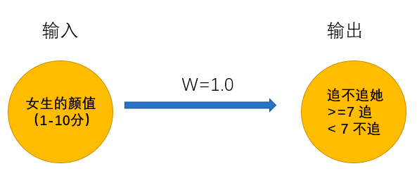
6. 神经网络示例
一个男孩想要找一个女朋友,于是实现了一个女友判定机,随着年龄的增长,他的判定机也一直在变化
14岁的时候:
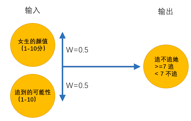
无数次碰壁之后,男孩意识到追到女孩的可能性和颜值一样重要,于是修改了判定机:
在15岁的时候终于找到呢女朋友,但是一顿时间后他发现有各种难以忍受的习惯,最终决定分手。一段空窗期中,他发现找女朋友很复杂,需要更多的条件才能够帮助他找到女朋友,于是在25岁的时候,他再次修改了判定机:
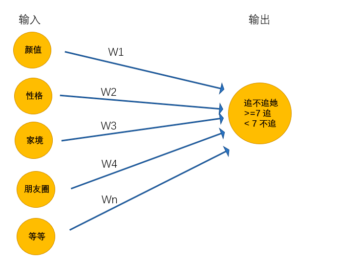
在更新了女友判定机之后,问题又来了,很多指标不能够很好的量化,如何颜值,什么样的叫做颜值高,什么样的叫做性格好等等,为了解决这个问题,他又更新了判定机,最终得到超级女友判定机
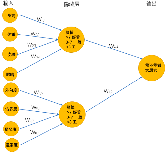
上述的超级女友判定机其实就是神经网络,它能够接受基础的输入,通过隐藏层的线性的和非线性的变化最终的到输出
通过上面例子,希望大家能够理解深度学习的思想:
输出的最原始、最基本的数据,通过模型来进行特征工程,进行更加高级特征的学习,然后通过传入的数据来确定合适的参数,让模型去更好的拟合数据。
这个过程可以理解为盲人摸象,多个人一起摸,把摸到的结果乘上合适的权重,进行合适的变化,让他和目标值趋近一致。整个过程只需要输入基础的数据,程序自动寻找合适的参数。
假设我们有这样一组数据,三角形和四边形,需要把他们分为两类
playground使用和演示
网址:http://playground.tensorflow.org
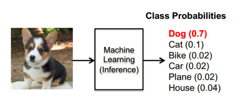
神经网络的主要用途在于分类,那么整个神经网络分类的原理是怎么样的?我们还是围绕着损失、优化这两块去说。神经网络输出结果如何分类?
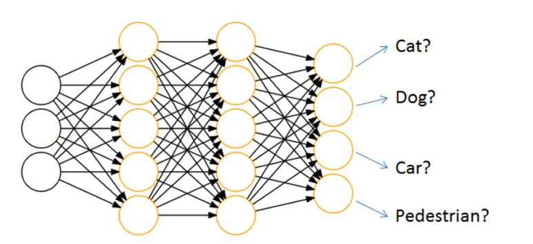
神经网络解决多分类问题最常用的方法是设置n个输出节点,其中n为类别的个数。
任意事件发生的概率都在0和1之间,且总有某一个事件发生(概率的和为1)。如果将分类问题中“一个样例属于某一个类别”看成一个概率事件,那么训练数据的正确答案就符合一个概率分布。如何将神经网络前向传播得到的结果也变成概率分布呢?Softmax回归就是一个非常常用的方法。
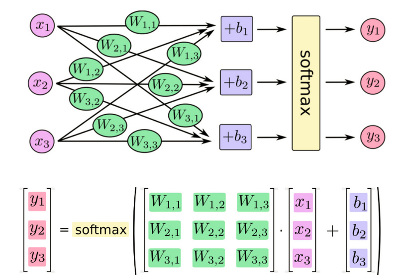
softmax回归
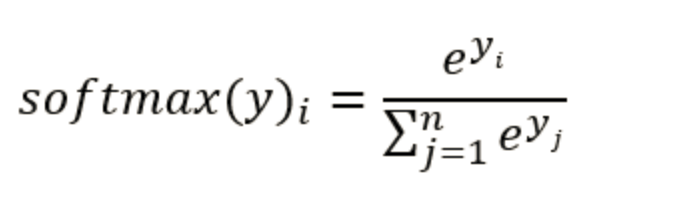
softmax特点
如何理解这个公式的作用呢?看一下计算案例
Softmax回归将神经网络输出转换成概率结果
假设输出结果为:2.3, 4.1, 5.6
softmax的计算输出结果为:
y1_p = e^2.3/(e^2.3+e^4.1+e^5.6)
y1_p = e^4.1/(e^2.3+e^4.1+e^5.6)
y1_p = e^5.6/(e^2.3+e^4.1+e^5.6)
这样就把神经网络的输出也变成了一个概率输出
类似于逻辑回归当中的sigmoid函数,sigmoid输出的是某个类别的概率
想一想线性回归的损失函数以及逻辑回归的损失函数,那么如何去衡量神经网络预测的概率分布和真实答案的概率分布之间的距离?
交叉熵损失
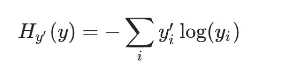
为了能够衡量距离,目标值需要进行one-hot编码,能与概率值一一对应,如下图
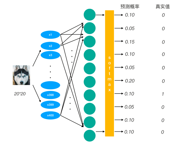
它的损失如何计算?
0log(0.10)+0log(0.05)+0log(0.15)+0log(0.10)+0log(0.05)+0log(0.20)+1log(0.10)+0log(0.05)+0log(0.10)+0log(0.10)
上述的结果为1log(0.10),那么为了减少这一个样本的损失。神经网络应该怎么做?所以会提高对应目标值为1的位置输出概率大小,由于softmax公式影响,其它的概率必定会减少。只要这样进行调整这样是不是就预测成功了!!!!!
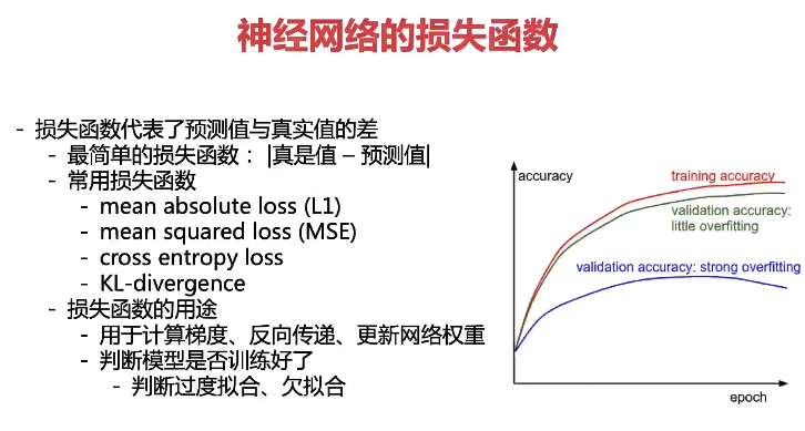
损失大小
神经网络最后的损失为平均每个样本的损失大小。对所有样本的损失求和取其平均值
有了这两个关键部分,神经网络的分类就是这样去做的,但是它是如何优化这些输出概率的呢?
BP算法(了解)(Backpropagation)
神经网络当中充满大量的权重、偏置参数,这些参数都需要去进行优化。之前我们接触的线性回归、逻辑回归通过梯度下降优化参数。这里也是一样,只不过由于神经网络的隐层可以增加很多层,那么这个过程需要一种规则。
定义:梯度下降+链式求导规则
BP算法过程
1、前向传输(Feed-Forward)
从输入层=>隐藏层=>输出层,一层一层的计算所有神经元输出值的过程。
2、逆向反馈(Back Propagation)
因为输出层的值与真实的值会存在误差,我们可以用均方误差来衡量预测值和真实值之间的误差。
- 在手工设定了神经网络的层数,每层的神经元的个数,学习率 η(下面会提到)后,BP 算法会先随机初始化每条连接线权重和偏置
- 对于训练集中的每个输入 x 和输出 y,BP 算法都会先执行前向传输得到预测值
- 根据真实值与预测值之间的误差执行逆向反馈更新神经网络中每条连接线的权重和每层的偏好。
我们不会详细地讨论可以如何使用反向传播和梯度下降等算法训练参数。训练过程中的计算机会尝试一点点增大或减小每个参数,看其能如何减少相比于训练数据集的误差,以望能找到最优的权重、偏置参数组合
案例: Pytorch+线性神经网络进行波士顿房价预测
- Pytorch下载
https://pytorch.org/get-started/locally/ 选择对应的版本命令

- 加载数据
import torch
import numpy as np
from sklearn import datasets
from sklearn.model_selection import train_test_split
from sklearn.preprocessing import StandardScaler
boston = datasets.load_boston()
X = boston.data
y = boston.target
X = X[y < 50.0]
y = y[y < 50.0]
X_train, X_test, y_train, y_test = train_test_split(X, y)
standardScaler = StandardScaler()
standardScaler.fit(X_train)
X_train = standardScaler.transform(X_train)
X_test = standardScaler.transform(X_test)
X_train.shape, X_test.shape, y_train.shape, y_test.shape
((367, 13), (123, 13), (367,), (123,))
- 训练
#net
class Net(torch.nn.Module):
    def __init__(self, n_feature, n_output):
        super(Net, self).__init__()
        self.hidden = torch.nn.Linear(n_feature, 100)
        self.predict = torch.nn.Linear(100, n_output)
    def forward(self, x):
        out = self.hidden(x)
        out = torch.relu(out)
        out = self.predict(out)
        return out
net = Net(13, 1)
#loss
loss_func = torch.nn.MSELoss()
#optimiter
optimizer = torch.optim.Adam(net.parameters(), lr=0.01)
#training
for i in range(10000):
x_data = torch.tensor(X_train, dtype=torch.float32)
y_data = torch.tensor(y_train, dtype=torch.float32)
pred = net.forward(x_data)
# squeeze(a)就是将a中所有为1的维度删掉
pred = torch.squeeze(pred)
loss = loss_func(pred, y_data) * 0.001
optimizer.zero_grad()
loss.backward()
optimizer.step()
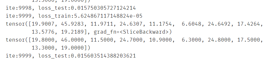
print("ite:{}, loss_train:{}".format(i, loss))
print(pred[0:10])
print(y_data[0:10])
#test
x_data = torch.tensor(X_test, dtype=torch.float32)
y_data = torch.tensor(y_test, dtype=torch.float32)
pred = net.forward(x_data)
pred = torch.squeeze(pred)
loss_test = loss_func(pred, y_data) * 0.001
print("ite:{}, loss_test:{}".format(i, loss_test))
torch.save(net, "boston_model.pkl")
- 加载模型测试
net = torch.load("boston_model.pkl")
loss_func = torch.nn.MSELoss()
#test
x_data = torch.tensor(X_test, dtype=torch.float32)
y_data = torch.tensor(y_test, dtype=torch.float32)
pred = net.forward(x_data)
pred = torch.squeeze(pred)
loss_test = loss_func(pred, y_data) * 0.001
print("loss_test:{}".format(loss_test))
loss_test:0.015603514388203621
线性神经网络局限性
任意多个隐层的神经网络和单层的神经网络都没有区别,而且都是线性的,而且线性模型的能够解决的问题也是有限的
神经网络的种类
- 基础神经网络:线性神经网络,BP神经网络,Hopfield神经网络等
- 进阶神经网络:玻尔兹曼机,受限玻尔兹曼机,递归神经网络等
- 深度神经网络:深度置信网络,卷积神经网络,循环神经网络,LSTM网络等
使用KreasAPI搭建神经网络
安装: https://tensorflow.google.cn/install
pip3 install --user --upgrade tensorflow
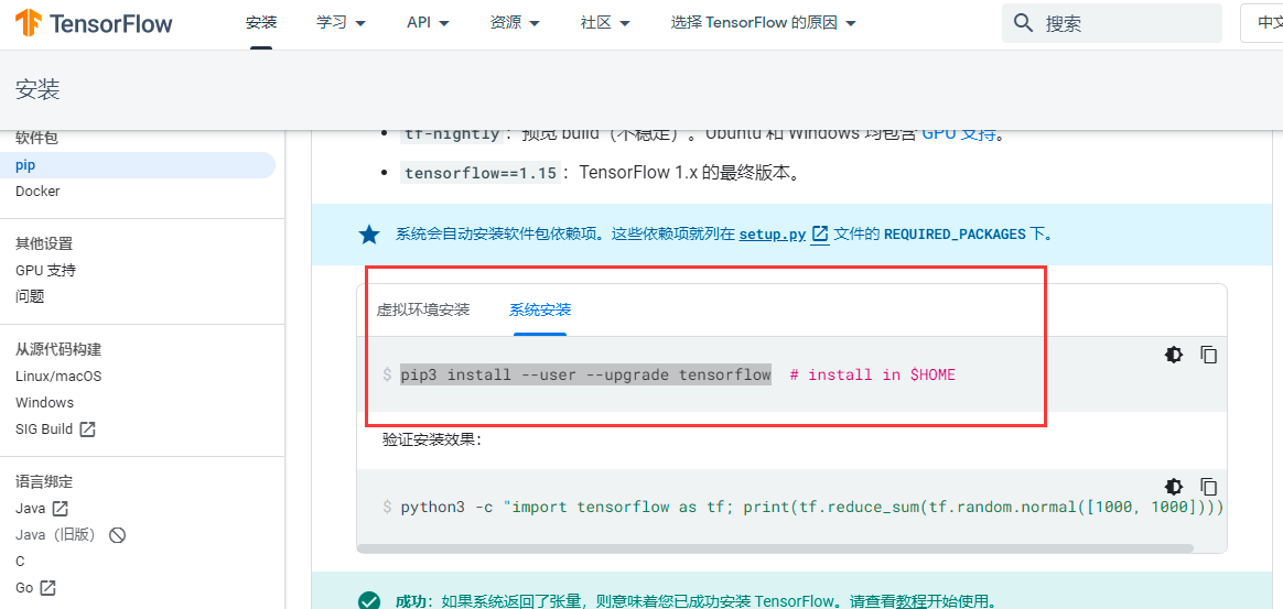
Keras是一个由Python编写的开源人工神经网络库,可以作为Tensorflow、Microsoft-CNTK和Theano的高阶应用程序接口,进行深度学习模型的设计、调试、评估、应用和可视化

#建立一个Sequential顺序模型
from keras.models import Sequential
model = Sequential()
Using TensorFlow backend.
#通过.add()叠加各层网络
# Dense即全连接层,逻辑上等价于这样一个函数:权重W为m*n的矩阵.输入x为n维向量.
# 激活函数Activation.偏置bias.输出向量out为m维向量.out=Activation(Wx+bias).
# 即一个线性变化加一个非线性变化产生输出.这是深度神经网络非常基本又十分强大的结构。
# 它的能力可以参考万能近似定理.很多其他的层,比如卷积层,都是在全连接的基础上加了很多先验形成的
from keras.layers import Dense
model.add(Dense(units=3, activation='sigmoid', input_dim=3))
model.add(Dense(units=1, activation='sigmoid'))
WARNING:tensorflow:From C:\Users\Eric\Anaconda3\lib\site-packages\tensorflow\python\framework\op_def_library.py:263: colocate_with (from tensorflow.python.framework.ops) is deprecated and will be removed in a future version.
Instructions for updating:
Colocations handled automatically by placer.
API 介绍
dense(
inputs,
units,
activation=None,
use_bias=True,
kernel_initializer=None,
bias_initializer=tf.zeros_initializer(),
kernel_regularizer=None,
bias_regularizer=None,
activity_regularizer=None,
trainable=True,
name=None,
reuse=None
)
- inputs: 输入数据,2维tensor.
- units: 该层的神经单元结点数。
- activation: 激活函数.
- use_bias: Boolean型,是否使用偏置项.
- kernel_initializer: 卷积核的初始化器.
- bias_initializer: 偏置项的初始化器,默认初始化为0.
- kernel_regularizer: 卷积核化的正则化,可选.
- bias_regularizer: 偏置项的正则化,可选.
- activity_regularizer: 输出的正则化函数.
- trainable: Boolean型,表明该层的参数是否参与训练。如果为真则变量加入到图集合中 GraphKeys.TRAINABLE_VARIABLES (see tf.Variable).
- name: 层的名字.
- reuse: Boolean型, 是否重复使用参数.
- 全连接层执行操作 outputs = activation(inputs.kernel+bias) 如果执行结果不想进行激活操作,则设置activation=None
#查看模型结构
model.summary()
Model: "sequential_1"
_________________________________________________________________
Layer (type)                 Output Shape              Param #
=================================================================
dense_1 (Dense)              (None, 3)                 12
_________________________________________________________________
dense_2 (Dense)              (None, 1)                 4
=================================================================
Total params: 16
Trainable params: 16
Non-trainable params: 0
_________________________________________________________________
#通过.compile()配置模型求解过程参数
# 交叉熵损失函数 categorical_crossentropy
model.compile(loss='categorical_crossentropy',
              optimizer='sgd',
              metrics=['accuracy'])
#训练模型
# model.fit(x_train, y_train, epochs=5)
构建多层感知机
好坏质检二分类mlp实战
1、通过mlp模型,在不增加特征项的情况下,实现了非线性二分类任务;
2、掌握了mlp模型的建立、配置与训练方法,并实现基于新数据的预测;
3、熟悉了mlp分类的预测数据格式,并实现格式转换;
4、核心算法参考链接:https://keras-cn.readthedocs.io/en/latest/#30sker
基于data.csv (链接:https://pan.baidu.com/s/1GoWnSt8ArNxa75mhys8Dnw
提取码:8888
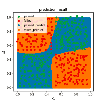
–来自百度网盘超级会员V5的分享)数据,建立mlp模型,计算其在测试数据上的准确率,可视化模型预测结果:
1.进行数据分离:test_size=0.33,random_state=10
2.模型结构:一层隐藏层,有20个神经元
#loada the data
import pandas as pd
import numpy as np
data = pd.read_csv('data.csv')
data.head()
| x1 | x2 | y | |
|---|---|---|---|
| 0 | 0.0323 | 0.0244 | 1 |
| 1 | 0.0887 | 0.0244 | 1 |
| 2 | 0.1690 | 0.0163 | 1 |
| 3 | 0.2420 | 0.0000 | 1 |
| 4 | 0.2420 | 0.0488 | 1 |
#define the X and y
X = data.drop(['y'],axis=1)
y = data.loc[:,'y']
X.head()
| x1 | x2 | |
|---|---|---|
| 0 | 0.0323 | 0.0244 |
| 1 | 0.0887 | 0.0244 |
| 2 | 0.1690 | 0.0163 |
| 3 | 0.2420 | 0.0000 |
| 4 | 0.2420 | 0.0488 |
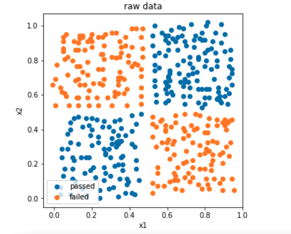
#visualize the data
%matplotlib inline
from matplotlib import pyplot as plt
fig1 = plt.figure(figsize=(5,5))
passed=plt.scatter(X.loc[:,'x1'][y==1],X.loc[:,'x2'][y==1])
failed=plt.scatter(X.loc[:,'x1'][y==0],X.loc[:,'x2'][y==0])
plt.legend((passed,failed),('passed','failed'))
plt.xlabel('x1')
plt.ylabel('x2')
plt.title('raw data')
plt.show()
#split the data
from sklearn.model_selection import train_test_split
X_train,X_test,y_train,y_test = train_test_split(X,y,test_size=0.33,random_state=10)
print(X_train.shape,X_test.shape,X.shape)
(275, 2) (136, 2) (411, 2)
#set up the model
from keras.models import Sequential
from keras.layers import Dense, Activation

mlp = Sequential()
mlp.add(Dense(units=20, input_dim=2, activation='sigmoid'))
mlp.add(Dense(units=1,activation='sigmoid'))
mlp.summary()
Using TensorFlow backend.


WARNING:tensorflow:From C:\Users\Eric\Anaconda3\lib\site-packages\tensorflow\python\framework\op_def_library.py:263: colocate_with (from tensorflow.python.framework.ops) is deprecated and will be removed in a future version.
Instructions for updating:
Colocations handled automatically by placer.
Model: "sequential_1"
_________________________________________________________________
Layer (type)                 Output Shape              Param #
=================================================================
dense_1 (Dense)              (None, 20)                60
_________________________________________________________________
dense_2 (Dense)              (None, 1)                 21
=================================================================
Total params: 81
Trainable params: 81
Non-trainable params: 0
_________________________________________________________________
#compile the model
# binary_crossentropy经常搭配sigmoid分类函数,categorical_crossentropy搭配softmax分类函数
# binary_crossentropy只能二分类
mlp.compile(optimizer='adam',loss='binary_crossentropy')
#train the model
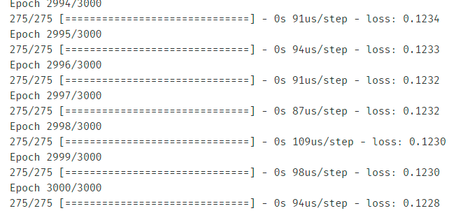
mlp.fit(X_train,y_train,epochs=3000)
WARNING:tensorflow:From C:\Users\Eric\Anaconda3\lib\site-packages\tensorflow\python\ops\math_ops.py:3066: to_int32 (from tensorflow.python.ops.math_ops) is deprecated and will be removed in a future version.
Instructions for updating:
Use tf.cast instead.
Epoch 1/3000
275/275 [==============================] - 1s 2ms/step - loss: 0.6932
Epoch 2/3000
275/275 [==============================] - 0s 94us/step - loss: 0.6927
Epoch 3/3000
275/275 [==============================] - 0s 94us/step - loss: 0.6926
Epoch 4/3000
275/275 [==============================] - 0s 94us/step - loss: 0.6925
Epoch 5/3000
275/275 [==============================] - 0s 98us/step - loss: 0.6925
Epoch 6/3000
275/275 [==============================] - 0s 83us/step - loss: 0.6926
Epoch 7/3000
275/275 [==============================] - 0s 91us/step - loss: 0.6924
Epoch 8/3000
275/275 [==============================] - 0s 101us/step - loss: 0.6923
Epoch 9/3000
275/275 [==============================] - 0s 94us/step - loss: 0.6924
Epoch 10/3000
#make prediction and calculate the accuracy
y_train_predict = mlp.predict_classes(X_train)
from sklearn.metrics import accuracy_score
accuracy_train = accuracy_score(y_train,y_train_predict)
print(accuracy_train)
0.9781818181818182
#make prediction based on the test data
y_test_predict = mlp.predict_classes(X_test)
accuracy_test = accuracy_score(y_test,y_test_predict)
print(accuracy_test)
0.9779411764705882
print(y_train_predict[0:10])
#y_train_predict_form = pd.Series(i[0] for i in y_train_predict)

#print(y_train_predict_form)
[[1]
 [0]
 [0]
 [0]
 [1]
 [0]
 [1]
 [1]
 [1]
 [1]]
#generate new data for plot
xx, yy = np.meshgrid(np.arange(0,1,0.01),np.arange(0,1,0.01))
x_range = np.c_[xx.ravel(),yy.ravel()]
y_range_predict = mlp.predict_classes(x_range)
print(type(y_range_predict))
<class 'numpy.ndarray'>
#format the output
y_range_predict_form = pd.Series(i[0] for i in y_range_predict)

print(y_range_predict_form)
0       1
1       1
2       1
3       1
4       1
       ..
9995    1
9996    1
9997    1
9998    1
9999    1
Length: 10000, dtype: int64
fig2 = plt.figure(figsize=(5,5))
passed_predict=plt.scatter(x_range[:,0][y_range_predict_form==1],x_range[:,1][y_range_predict_form==1])
failed_predict=plt.scatter(x_range[:,0][y_range_predict_form==0],x_range[:,1][y_range_predict_form==0])

passed=plt.scatter(X.loc[:,'x1'][y==1],X.loc[:,'x2'][y==1])
failed=plt.scatter(X.loc[:,'x1'][y==0],X.loc[:,'x2'][y==0])
plt.legend((passed,failed,passed_predict,failed_predict),('passed','failed','passed_predict','failed_predict'))
plt.xlabel('x1')
plt.ylabel('x2')
plt.title('prediction result')
plt.show()
好坏质检二分类mlp实战summary:
1、通过mlp模型,在不增加特征项的情况下,实现了非线性二分类任务;
2、掌握了mlp模型的建立、配置与训练方法,并实现基于新数据的预测;
3、熟悉了mlp分类的预测数据格式,并实现格式转换;
4、核心算法参考链接:https://keras-cn.readthedocs.io/en/latest/#30skeras
手写数字识别
基于mnist数据集,建立mlp模型,实现0-9数字的十分类task::
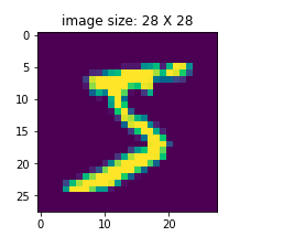
1.实现mnist数据载入,可视化图形数字
2.完成数据预处理:图像数据维度转换与归一化、输出结果格式转换
3.计算模型在预测数据集的准确率
4.模型结构:两层隐藏层,每层有392个神经元
# load the mnist data
from keras.datasets import mnist
(X_train,y_train),(X_test,y_test) = mnist.load_data()
Using TensorFlow backend.
print(type(X_train),X_train.shape)
<class 'numpy.ndarray'> (60000, 28, 28)
#visualize the data
img1 = X_train[0]
%matplotlib inline
from matplotlib import pyplot as plt
fig1 = plt.figure(figsize=(3,3))
plt.imshow(img1)
plt.title('image size: 28 X 28')
plt.show()
img1
array([[  0,   0,   0,   0,   0,   0,   0,   0,   0,   0,   0,   0,   0,
          0,   0,   0,   0,   0,   0,   0,   0,   0,   0,   0,   0,   0,
          0,   0],
       [  0,   0,   0,   0,   0,   0,   0,   0,   0,   0,   0,   0,   0,
          0,   0,   0,   0,   0,   0,   0,   0,   0,   0,   0,   0,   0,
          0,   0],
       [  0,   0,   0,   0,   0,   0,   0,   0,   0,   0,   0,   0,   0,
          0,   0,   0,   0,   0,   0,   0,   0,   0,   0,   0,   0,   0,
          0,   0],
       [  0,   0,   0,   0,   0,   0,   0,   0,   0,   0,   0,   0,   0,
          0,   0,   0,   0,   0,   0,   0,   0,   0,   0,   0,   0,   0,
          0,   0],
       [  0,   0,   0,   0,   0,   0,   0,   0,   0,   0,   0,   0,   0,
          0,   0,   0,   0,   0,   0,   0,   0,   0,   0,   0,   0,   0,
          0,   0],
       [  0,   0,   0,   0,   0,   0,   0,   0,   0,   0,   0,   0,   3,
         18,  18,  18, 126, 136, 175,  26, 166, 255, 247, 127,   0,   0,
          0,   0],
       [  0,   0,   0,   0,   0,   0,   0,   0,  30,  36,  94, 154, 170,
        253, 253, 253, 253, 253, 225, 172, 253, 242, 195,  64,   0,   0,
          0,   0],
       [  0,   0,   0,   0,   0,   0,   0,  49, 238, 253, 253, 253, 253,
        253, 253, 253, 253, 251,  93,  82,  82,  56,  39,   0,   0,   0,
          0,   0],
       [  0,   0,   0,   0,   0,   0,   0,  18, 219, 253, 253, 253, 253,
        253, 198, 182, 247, 241,   0,   0,   0,   0,   0,   0,   0,   0,
          0,   0],
       [  0,   0,   0,   0,   0,   0,   0,   0,  80, 156, 107, 253, 253,
        205,  11,   0,  43, 154,   0,   0,   0,   0,   0,   0,   0,   0,
          0,   0],
       [  0,   0,   0,   0,   0,   0,   0,   0,   0,  14,   1, 154, 253,
         90,   0,   0,   0,   0,   0,   0,   0,   0,   0,   0,   0,   0,
          0,   0],
       [  0,   0,   0,   0,   0,   0,   0,   0,   0,   0,   0, 139, 253,
        190,   2,   0,   0,   0,   0,   0,   0,   0,   0,   0,   0,   0,
          0,   0],
       [  0,   0,   0,   0,   0,   0,   0,   0,   0,   0,   0,  11, 190,
        253,  70,   0,   0,   0,   0,   0,   0,   0,   0,   0,   0,   0,
          0,   0],
       [  0,   0,   0,   0,   0,   0,   0,   0,   0,   0,   0,   0,  35,
        241, 225, 160, 108,   1,   0,   0,   0,   0,   0,   0,   0,   0,
          0,   0],
       [  0,   0,   0,   0,   0,   0,   0,   0,   0,   0,   0,   0,   0,
         81, 240, 253, 253, 119,  25,   0,   0,   0,   0,   0,   0,   0,
          0,   0],
       [  0,   0,   0,   0,   0,   0,   0,   0,   0,   0,   0,   0,   0,
          0,  45, 186, 253, 253, 150,  27,   0,   0,   0,   0,   0,   0,
          0,   0],
       [  0,   0,   0,   0,   0,   0,   0,   0,   0,   0,   0,   0,   0,
          0,   0,  16,  93, 252, 253, 187,   0,   0,   0,   0,   0,   0,
          0,   0],
       [  0,   0,   0,   0,   0,   0,   0,   0,   0,   0,   0,   0,   0,
          0,   0,   0,   0, 249, 253, 249,  64,   0,   0,   0,   0,   0,
          0,   0],
       [  0,   0,   0,   0,   0,   0,   0,   0,   0,   0,   0,   0,   0,
          0,  46, 130, 183, 253, 253, 207,   2,   0,   0,   0,   0,   0,
          0,   0],
       [  0,   0,   0,   0,   0,   0,   0,   0,   0,   0,   0,   0,  39,
        148, 229, 253, 253, 253, 250, 182,   0,   0,   0,   0,   0,   0,
          0,   0],
       [  0,   0,   0,   0,   0,   0,   0,   0,   0,   0,  24, 114, 221,
        253, 253, 253, 253, 201,  78,   0,   0,   0,   0,   0,   0,   0,
          0,   0],
       [  0,   0,   0,   0,   0,   0,   0,   0,  23,  66, 213, 253, 253,
        253, 253, 198,  81,   2,   0,   0,   0,   0,   0,   0,   0,   0,
          0,   0],
       [  0,   0,   0,   0,   0,   0,  18, 171, 219, 253, 253, 253, 253,
        195,  80,   9,   0,   0,   0,   0,   0,   0,   0,   0,   0,   0,
          0,   0],
       [  0,   0,   0,   0,  55, 172, 226, 253, 253, 253, 253, 244, 133,
         11,   0,   0,   0,   0,   0,   0,   0,   0,   0,   0,   0,   0,
          0,   0],
       [  0,   0,   0,   0, 136, 253, 253, 253, 212, 135, 132,  16,   0,
          0,   0,   0,   0,   0,   0,   0,   0,   0,   0,   0,   0,   0,
          0,   0],
       [  0,   0,   0,   0,   0,   0,   0,   0,   0,   0,   0,   0,   0,
          0,   0,   0,   0,   0,   0,   0,   0,   0,   0,   0,   0,   0,
          0,   0],
       [  0,   0,   0,   0,   0,   0,   0,   0,   0,   0,   0,   0,   0,
          0,   0,   0,   0,   0,   0,   0,   0,   0,   0,   0,   0,   0,
          0,   0],
       [  0,   0,   0,   0,   0,   0,   0,   0,   0,   0,   0,   0,   0,
          0,   0,   0,   0,   0,   0,   0,   0,   0,   0,   0,   0,   0,
          0,   0]], dtype=uint8)
#format the input data
feature_size = img1.shape[0]*img1.shape[1]
X_train_format = X_train.reshape(X_train.shape[0],feature_size)
X_test_format = X_test.reshape(X_test.shape[0],feature_size)


print(X_train_format.shape)
(60000, 784)
#normalize the input data
X_train_normal = X_train_format/255
X_test_normal = X_test_format/255
print(X_train_normal[0])
[0.         0.         0.         0.         0.         0.
 0.         0.         0.         0.         0.         0.
 0.         0.         0.         0.         0.         0.
 0.         0.         0.         0.         0.         0.
 0.         0.         0.         0.         0.         0.
 0.         0.         0.         0.         0.         0.
 0.         0.         0.         0.         0.         0.
 0.         0.         0.         0.         0.         0.
 0.         0.         0.         0.         0.         0.
 0.         0.         0.         0.         0.         0.
 0.         0.         0.         0.         0.         0.
 0.         0.         0.         0.         0.         0.
 0.         0.         0.         0.         0.         0.
 0.         0.         0.         0.         0.         0.
 0.         0.         0.         0.         0.         0.
 0.         0.         0.         0.         0.         0.
 0.         0.         0.         0.         0.         0.
 0.         0.         0.         0.         0.         0.
 0.         0.         0.         0.         0.         0.
 0.         0.         0.         0.         0.         0.
 0.         0.         0.         0.         0.         0.
 0.         0.         0.         0.         0.         0.
 0.         0.         0.         0.         0.         0.
 0.         0.         0.         0.         0.         0.
 0.         0.         0.         0.         0.         0.
 0.         0.         0.01176471 0.07058824 0.07058824 0.07058824
 0.49411765 0.53333333 0.68627451 0.10196078 0.65098039 1.
 0.96862745 0.49803922 0.         0.         0.         0.
 0.         0.         0.         0.         0.         0.
 0.         0.         0.11764706 0.14117647 0.36862745 0.60392157
 0.66666667 0.99215686 0.99215686 0.99215686 0.99215686 0.99215686
 0.88235294 0.6745098  0.99215686 0.94901961 0.76470588 0.25098039
 0.         0.         0.         0.         0.         0.
 0.         0.         0.         0.         0.         0.19215686
 0.93333333 0.99215686 0.99215686 0.99215686 0.99215686 0.99215686
 0.99215686 0.99215686 0.99215686 0.98431373 0.36470588 0.32156863
 0.32156863 0.21960784 0.15294118 0.         0.         0.
 0.         0.         0.         0.         0.         0.
 0.         0.         0.         0.07058824 0.85882353 0.99215686
 0.99215686 0.99215686 0.99215686 0.99215686 0.77647059 0.71372549
 0.96862745 0.94509804 0.         0.         0.         0.
 0.         0.         0.         0.         0.         0.
 0.         0.         0.         0.         0.         0.
 0.         0.         0.31372549 0.61176471 0.41960784 0.99215686
 0.99215686 0.80392157 0.04313725 0.         0.16862745 0.60392157
 0.         0.         0.         0.         0.         0.
 0.         0.         0.         0.         0.         0.
 0.         0.         0.         0.         0.         0.
 0.         0.05490196 0.00392157 0.60392157 0.99215686 0.35294118
 0.         0.         0.         0.         0.         0.
 0.         0.         0.         0.         0.         0.
 0.         0.         0.         0.         0.         0.
 0.         0.         0.         0.         0.         0.
 0.         0.54509804 0.99215686 0.74509804 0.00784314 0.
 0.         0.         0.         0.         0.         0.
 0.         0.         0.         0.         0.         0.
 0.         0.         0.         0.         0.         0.
 0.         0.         0.         0.         0.         0.04313725
 0.74509804 0.99215686 0.2745098  0.         0.         0.
 0.         0.         0.         0.         0.         0.
 0.         0.         0.         0.         0.         0.
 0.         0.         0.         0.         0.         0.
 0.         0.         0.         0.         0.1372549  0.94509804
 0.88235294 0.62745098 0.42352941 0.00392157 0.         0.
 0.         0.         0.         0.         0.         0.
 0.         0.         0.         0.         0.         0.
 0.         0.         0.         0.         0.         0.
 0.         0.         0.         0.31764706 0.94117647 0.99215686
 0.99215686 0.46666667 0.09803922 0.         0.         0.
 0.         0.         0.         0.         0.         0.
 0.         0.         0.         0.         0.         0.
 0.         0.         0.         0.         0.         0.
 0.         0.         0.17647059 0.72941176 0.99215686 0.99215686
 0.58823529 0.10588235 0.         0.         0.         0.
 0.         0.         0.         0.         0.         0.
 0.         0.         0.         0.         0.         0.
 0.         0.         0.         0.         0.         0.
 0.         0.0627451  0.36470588 0.98823529 0.99215686 0.73333333
 0.         0.         0.         0.         0.         0.
 0.         0.         0.         0.         0.         0.
 0.         0.         0.         0.         0.         0.
 0.         0.         0.         0.         0.         0.
 0.         0.97647059 0.99215686 0.97647059 0.25098039 0.
 0.         0.         0.         0.         0.         0.
 0.         0.         0.         0.         0.         0.
 0.         0.         0.         0.         0.         0.
 0.         0.         0.18039216 0.50980392 0.71764706 0.99215686
 0.99215686 0.81176471 0.00784314 0.         0.         0.
 0.         0.         0.         0.         0.         0.
 0.         0.         0.         0.         0.         0.
 0.         0.         0.         0.         0.15294118 0.58039216
 0.89803922 0.99215686 0.99215686 0.99215686 0.98039216 0.71372549
 0.         0.         0.         0.         0.         0.
 0.         0.         0.         0.         0.         0.
 0.         0.         0.         0.         0.         0.
 0.09411765 0.44705882 0.86666667 0.99215686 0.99215686 0.99215686
 0.99215686 0.78823529 0.30588235 0.         0.         0.
 0.         0.         0.         0.         0.         0.
 0.         0.         0.         0.         0.         0.
 0.         0.         0.09019608 0.25882353 0.83529412 0.99215686
 0.99215686 0.99215686 0.99215686 0.77647059 0.31764706 0.00784314
 0.         0.         0.         0.         0.         0.
 0.         0.         0.         0.         0.         0.
 0.         0.         0.         0.         0.07058824 0.67058824
 0.85882353 0.99215686 0.99215686 0.99215686 0.99215686 0.76470588
 0.31372549 0.03529412 0.         0.         0.         0.
 0.         0.         0.         0.         0.         0.
 0.         0.         0.         0.         0.         0.
 0.21568627 0.6745098  0.88627451 0.99215686 0.99215686 0.99215686
 0.99215686 0.95686275 0.52156863 0.04313725 0.         0.
 0.         0.         0.         0.         0.         0.
 0.         0.         0.         0.         0.         0.
 0.         0.         0.         0.         0.53333333 0.99215686
 0.99215686 0.99215686 0.83137255 0.52941176 0.51764706 0.0627451
 0.         0.         0.         0.         0.         0.
 0.         0.         0.         0.         0.         0.
 0.         0.         0.         0.         0.         0.
 0.         0.         0.         0.         0.         0.
 0.         0.         0.         0.         0.         0.
 0.         0.         0.         0.         0.         0.
 0.         0.         0.         0.         0.         0.
 0.         0.         0.         0.         0.         0.
 0.         0.         0.         0.         0.         0.
 0.         0.         0.         0.         0.         0.
 0.         0.         0.         0.         0.         0.
 0.         0.         0.         0.         0.         0.
 0.         0.         0.         0.         0.         0.
 0.         0.         0.         0.         0.         0.
 0.         0.         0.         0.         0.         0.
 0.         0.         0.         0.         0.         0.
 0.         0.         0.         0.        ]
# 对标签进行one hot编码 独热
# from tensorflow.keras.utils import to_categorical
y_train = tf.one_hot(indices=y_train, depth=10, on_value=1, off_value=0,axis=1)
y_test = tf.one_hot(indices=y_test, depth=10, on_value=1, off_value=0,axis=1)
print(X_train_normal.shape,y_train_format.shape)
(60000, 784) (60000, 10)
#set up the model
from keras.models import Sequential
from keras.layers import Dense, Activation

mlp = Sequential()
mlp.add(Dense(units=392,activation='relu',input_dim=784))
mlp.add(Dense(units=392,activation='relu'))
mlp.add(Dense(units=10,activation='softmax'))
mlp.summary()
WARNING:tensorflow:From C:\Users\Eric\Anaconda3\lib\site-packages\tensorflow\python\framework\op_def_library.py:263: colocate_with (from tensorflow.python.framework.ops) is deprecated and will be removed in a future version.
Instructions for updating:
Colocations handled automatically by placer.
Model: "sequential_1"
_________________________________________________________________
Layer (type)                 Output Shape              Param #
=================================================================
dense_1 (Dense)              (None, 392)               307720
_________________________________________________________________
dense_2 (Dense)              (None, 392)               154056
_________________________________________________________________
dense_3 (Dense)              (None, 10)                3930
=================================================================
Total params: 465,706
Trainable params: 465,706
Non-trainable params: 0
_________________________________________________________________
#configure the model
mlp.compile(loss='categorical_crossentropy',optimizer='adam',metrics=['categorical_accuracy'])
#train the model
mlp.fit(X_train_normal,y_train_format,epochs=10)
WARNING:tensorflow:From C:\Users\Eric\Anaconda3\lib\site-packages\tensorflow\python\ops\math_ops.py:3066: to_int32 (from tensorflow.python.ops.math_ops) is deprecated and will be removed in a future version.
Instructions for updating:
Use tf.cast instead.
Epoch 1/10
60000/60000 [==============================] - 51s 857us/step - loss: 0.1879 - categorical_accuracy: 0.9431 51s - loss: 0.3920 - categorical_accur - ETA: 50s - loss: 0.3800 - categori - ETA: 41s - loss: 0.3229 - categorical_accuracy:  - ETA: 41s -
Epoch 2/10
60000/60000 [==============================] - 53s 877us/step - loss: 0.0825 - categorical_accuracy: 0.9742 40s - lo - ETA: 39s - loss: 0.0823 - categor - ETA: 37s - loss: 0.0828 - categorical_accuracy - ETA: 36s - loss - ETA: 34s - loss: 0.0859 - categorical_accuracy: 0.973 - ETA: 34s - loss: 0.0856 - categorical_accuracy: 0 - ETA: 33s - loss: 0.0853 - categorical_accuracy:  - ETA: 3 - ETA: 3 - ETA - ETA: 18s - los
Epoch 3/10
60000/60000 [==============================] - 46s 759us/step - loss: 0.0553 - categorical_accuracy: 0.9824s - loss: 0.0557 - catego
Epoch 4/10
60000/60000 [==============================] - 40s 674us/step - loss: 0.0432 - categorical_accuracy: 0.9863 49s - loss: 0.0286  - ETA: 47s - loss: 0.0310 - ETA: 39s - loss: 0.0333 - categorical_ac - - ETA: 1s - loss: 0.042
Epoch 5/10
60000/60000 [==============================] - 33s 546us/step - loss: 0.0343 - categorical_accuracy: 0.9889 26s - loss: 0.0253 - categorical_accuracy: 0.992 - - ETA: 11s - loss: 0.0298 - categorical_accuracy: - ETA: 8s - los - - ETA: 2s - ETA: 1s -
Epoch 6/10
60000/60000 [==============================] - 33s 547us/step - loss: 0.0286 - categorical_accuracy: 0.9909s - loss: 0.0272 -  - ETA: 0s - loss: 0.0287 - categorica
Epoch 7/10
60000/60000 [==============================] - 34s 565us/step - loss: 0.0242 - categorical_accuracy: 0.9927 30s - loss: 0.0186 - categorical_accuracy: 0 - ETA: 30s - loss: 0.0187 - categorical_accuracy: 0.993 - ETA: 30s -
Epoch 8/10
60000/60000 [==============================] - 33s 557us/step - loss: 0.0226 - categorical_accuracy: 0.9930
Epoch 9/10
60000/60000 [==============================] - 33s 547us/step - loss: 0.0175 - categorical_accuracy: 0.9945 29s - loss: 0 - ETA: 22s - loss: 0.0106 - ETA: 20s - loss: 0.0126 - categorical_accuracy: 0. - ETA: 19s - - ETA: 17s - loss: 0.0152 - categor - ETA: 13s - loss: 0.0168 - categorical_accuracy: 0.994 - ETA: 12s - loss: 0.0168 -  - ET - ETA: 9s - ETA: 1s - loss: - ETA: 0s - loss: 0.0175 - categorical_accuracy: 0.99
Epoch 10/10
60000/60000 [==============================] - 33s 548us/step - loss: 0.0179 - categorical_accuracy: 0.9941s - loss: 0.0178 - categorical_accuracy: 0.99 - ETA: 1s - loss: 0.017 - ETA: 0s - loss: 0.0178 -


<keras.callbacks.History at 0x1b539bbae48>
#evaluate the model
y_train_predict = mlp.predict_classes(X_train_normal)
print(type(y_train_predict))
<class 'numpy.ndarray'>
print(y_train_predict[0:10])
[5 0 4 1 9 2 1 3 1 4]
from sklearn.metrics import accuracy_score
accuracy_train = accuracy_score(y_train,y_train_predict)
print(accuracy_train)
0.9948166666666667
y_test_predict = mlp.predict_classes(X_test_normal)
accuracy_test = accuracy_score(y_test,y_test_predict)
print(accuracy_test)
0.9799
img2 = X_test[100]
fig2 = plt.figure(figsize=(3,3))
plt.imshow(img2)
plt.title(y_test_predict[100])
plt.show()
![[外链图片转存失败,源站可能有防盗链机制,建议将图片保存下来直接上传(img-C3fgbqJw-1632291648082)(output_17_0.png)]](https://img-blog.csdnimg.cn/0f2e4a4125704358a425b9e5c929e8af.png)
# coding:utf-8
import matplotlib as mlp
font2 = {'family' : 'SimHei',
'weight' : 'normal',
'size' : 20,
}
mlp.rcParams['font.family'] = 'SimHei'
mlp.rcParams['axes.unicode_minus'] = False
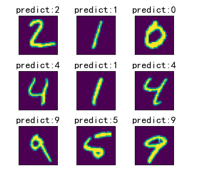
a = [i for i in range(1,10)]
fig4 = plt.figure(figsize=(5,5))
for i in a:
plt.subplot(3,3,i)
plt.tight_layout()
plt.imshow(X_test[i])
plt.title('predict:{}'.format(y_test_predict[i]),font2)
plt.xticks([])
plt.yticks([])
# 加载mnist数据集
import tensorflow as tf
from keras.datasets import mnist
(X_train, y_train),  (X_test, y_test) = mnist.load_data()

# 随机选一张
# six = X_train[12]
# # print(six)
# for row in six:
#     for v in row :
#         print(v, end="\t")
#     print()
# from matplotlib import pyplot as plt
# plt.imshow(six, cmap='gray')
# plt.show()
# print(y_train[12]) #
# 整理数据
X_train = X_train.reshape(60000, 784)
X_test = X_test.reshape(10000, 784)
# 归一化
X_train = X_train/255
X_test = X_test/255
# 对标签进行one hot编码 独热

y_train = tf.one_hot(indices=y_train,
                     depth=10, on_value=1, off_value=0,axis=1)
y_test = tf.one_hot(indices=y_test, depth=10, on_value=1, off_value=0,axis=1)
y_train =y_train.numpy()
y_test =y_test.numpy()
print(X_train.shape)
print(y_train.shape)
print(X_test.shape)
print(y_test.shape)
print(y_train[12])
# 搭建神经网络
from keras.models import Sequential
from keras.layers import Dense
import numpy as np
mlp = Sequential()
mlp.add(Dense(units=400, input_dim=784, activation='relu'))
mlp.add(Dense(units=400, activation='relu'))
mlp.add(Dense(units=10, activation='softmax'))
mlp.summary()
mlp.compile(optimizer='adam', loss='categorical_crossentropy', metrics=['categorical_accuracy'])
mlp.fit(X_train, y_train, epochs=10)
y_pred = mlp.predict(X_test)
y_pred1 = np.argmax(y_pred, axis=1)
# print(y_pred)
print(y_pred1[:10])
print("----")
y_test = np.argmax(y_test, axis=1)
print(y_test[:10])

scores = sum(y_pred1 == y_test)/len(y_test)
print(scores)
图像数字多分类实战summary:
1、通过mlp模型,实现了基于图像数据的数字自动识别分类;
2、完成了图像的数字化处理与可视化;
3、对mlp模型的输入、输出数据格式有了更深的认识,完成了数据预处理与格式转换;
4、建立了结构更为复杂的mlp模型
5、mnist数据集地址:http://yann.lecun.com/exdb/mnist/
作业
基于fashion_mnist数据集,建立mlp模型,实现服饰图片十分类。
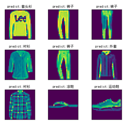
图片描述
1、实现图像数据加载、可视化
2、进行数据预处理:维度转化,归一化、输出结果格式转化
3、建立mlp模型,进行模型训练与预测,计算模型在训练、测试数据集的准确率
4、选取一个测试样本,预测其类别
5、选取测试集前10个样本,分别预测其类别
提示:
模型结构:两层隐藏层(激活函数:relu),分别有392、196个神经元;输出层10类,激活函数softmax
提示2:
一个替代MNIST手写数字集的图像数据集, 涵盖了来自10种类别的共7万个不同服饰商品的正面图片,由60000个训练样本和10000个测试样本组成,每个样本都是一张28 * 28像素的灰度图片。
官方网站 :
https://github.com/zalandoresearch/fashion-mnist
一共4个文件,训练集、训练集标签、测试集、测试集标签
#图像加载与展示
from keras.datasets import fashion_mnist
(X_train, y_train), (X_test, y_test) = fashion_mnist.load_data()
print(type(X_train),’\n’,X_train.shape)
https://blog.csdn.net/u013705056/article/details/110819827?utm_medium=distribute.pc_relevant.none-task-blog-2%7Edefault%7ECTRLIST%7Edefault-4.no_search_link&depth_1-utm_source=distribute.pc_relevant.none-task-blog-2%7Edefault%7ECTRLIST%7Edefault-4.no_search_link